Here are the slides I presented for a ClickHouse SF Bay Area Meetup in July 2022, hosted by Altinity. They are about Akvorado, a network flow collector and visualizer, and notably on how it relies on ClickHouse, a column-oriented database.

The meetup was recorded and available on YouTube. Here is the part relevant to my presentation, with subtitles:¹

I got a few questions about how to get information from the higher layers, like HTTP. As my use case for Akvorado was at the network edge, my answers were mostly negative. However, as sFlow is extensible, when collecting flows from Linux servers instead, you could embed additional data and they could be exported as well.

I also got a question about doing aggregation in a single table. ClickHouse can automatically aggregate data using TTL. My answer for not doing that is partial. There is another reason: the retention periods of the various tables may overlap. For example, the main table keeps data for 15 days, but even in these 15 days, if I do a query on a 12-hour window, it is faster to use the flows_1m0s aggregated table, unless I request something about ports and IP addresses.

Transcript#

Hello. So I am Vincent Bernat. I’m a French network engineer working at Free. I’m doing this presentation from Paris, France. So it’s nice to see you. I’m going to present Akvorado, a network flow collector and visualizer backed by ClickHouse.

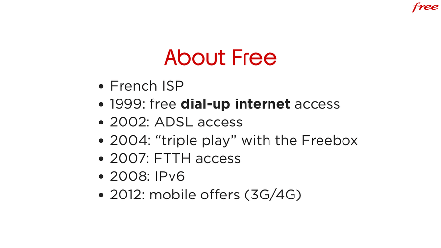
It was developed internally at Free. Free is a French ISP founded in 1999. It was one of the first to offer internet access without a subscription or surcharged phone number in France. It contributed to the DSL expansion in France by driving prices down. It was quite innovative by introducing the Freebox. This is the first triple play setup box including Internet, TV and phone services. It also contributed a lot to the IPv6 adoption in France in 2008. The mobile offer is also quite innovative with the big data allowance. You have more than 100 GB of data included and you can roam in the world with that but we are not available in San Francisco yet.

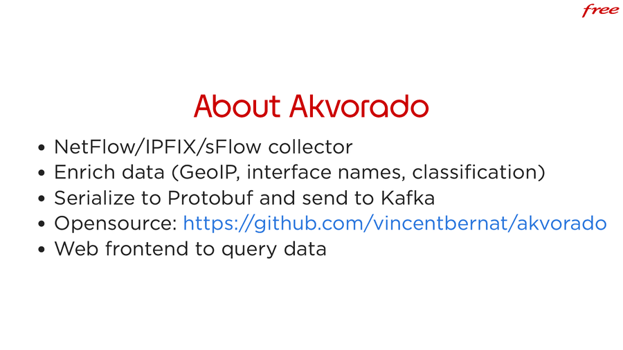
So Akvorado is a NetFlow, IPFIX, sFlow collector. Internet routers send a sample of the packets they received to Akvorado, like one packet out of 10,000.

There are several protocols for that. IPFIX is the IETF version of NetFlow. NetFlow is Cisco proprietary protocol. sFlow is another kind of protocol. The difference is that it does not aggregate data. It sends data in real time. But it’s a small difference because NetFlow is also able to send data almost in realtime with a good configuration. You can have a 10s lag. So mostly you choose the protocol that your router support. So it’s important to support several protocols because not all routers support all protocols.

So Akvorado receives that and then it enriches the flow with additional data. Notably it adds GeoIP information using the MaxMind databases, add interface names and descriptions with the SNMP protocol and it adds AS numbers. AS numbers are the main way to identify organization on the internet. From the IP address, you can get the AS number and from the AS number you can get the name.

We also add some attributes to the routers using classification rules: we add the location, the role, the tenant of the router and we also add attributes to interfaces: the provider, the boundary, the connectivity (is it the transit interface or a peering interface). All this information are very useful to have when you need to query the data that you’ve collected.

And then, Akvorado will serialize the flow using Protobuf and send that to a Kafka cluster. Since recently, this is an open source project. We have published it on GitHub. There is also a nice web frontend to query the data.

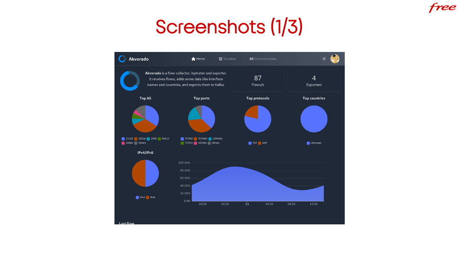
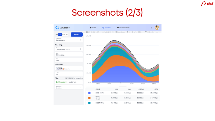
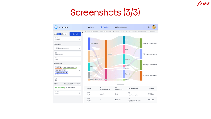
Here are a few screenshot but I will do a live demo.

You can try the demo yourself. The URL is demo.akvorado.net. It’s running on a small virtual machine. It uses fake data.

The home page is just a few metrics to show that it works correctly but it also displays the last received flow. You can see what it looks like. You have a time stamp, the number of bytes, the number of packets, the router that sent the flow. Its name.

The following attributes come from the classification rules. The sampling rate, which is quite high for the demo. It means that the router sent one flow out of 50,000 flows it received. The source address. The source AS number. GeoIP is not configured so they don’t get the country. You get the source port.

As for the incoming interface, you get the name, the description, the speed and also from the classification rules the fact that it’s an external facing interface (it’s connected to the internet). It’s a transit interface connected to Cogent which is a transit provider and you have the same stuff for the destination address, the country, and the outgoing interface.

We have EType which is mostly IPv4 or IPv6. Forwarding status. 64 means it has been forwarded. 128 means the packet has been dropped. So if you have firewall rules it’s interesting. And the protocol: it’s 17 for UDP, 6 for TCP. So most of the fields were received from the flow but some of them were added later.

Okay. But the most interesting tab is visualize tab. Let me zoom back a bit to show the last seven days. So it answers the question “where does my traffic come from?” We can see for example in this demo that most of the traffic comes from Netflix but also Google and Facebook. There is a filter and you can add more stuff like, for example, I want to only see the IPv6 traffic. I can input this filter and when I apply, I get the IPv6 traffic. Because all the data is fake it’s a bit difficult to see the difference but you see IPv6 is at most 60Gbps of traffic while the whole traffic was about 90 Gbps.

Another interesting visualization that the web interface shows is a sankey graph. It’s another kind of visualization and it shows us the top three talkers: Netflix, Google and Facebook. It shows that two thirds of the traffic is going through transit providers. One third is going through internet exchanges.

Internet exchange is a place where people can connect to the same switch and exchange traffic for free or not. But you don’t get the whole internet just by going to an internet exchange. If you want to get the whole internet you need to have a transit provider.

So for example, we can answer the question “How do we get google traffic?” It seems that you get most of the traffic using a transit provider but a small part is going through an internet exchange. It’s also very useful visualization to get for a network engineer. Let me get back to the presentation.

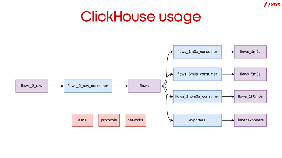
How did we use ClickHouse? So that’s the tables that we have in our setup. First a bit of warning. It’s the first time I have used ClickHouse. I am a network engineer, not a database engineer. I have a few notions of database but very light. So feedback is welcome and take everything with a grain of salt.

So the purple squares are the tables, the blue ones are the views and the white one are the dictionaries. I was too fast. I think I forgot to tell… No, no. Okay, sorry. So like I told previously, flows are coming from Kafka on the flows_2_raw table which is not backed by disk storage. There is the consumer extracting the flows and sending them to the flows table which is the main table containing all the flows. Then we have a few other flow tables which are aggregating data over time to take less space and speed up queries. I will go in more details in the next slides.

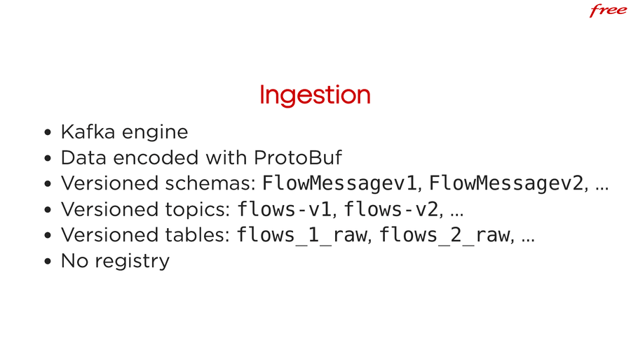
So ingestion is done using the Kafka engine. We receive the data using the Kafka engine. The data is decoded with the Protobuf format. Protobuf schemas are versioned. They are coming from versioned topics from Kafka and stored in versioned tables.

The flows table itself is not versioned. The flows consumer will normalize data to match the data format in the flows table. When there is a schema change, we increase the version number. It allows seamless updates. If you have old collectors running in your network, they still work. For example, they will continue to send the flows to the flows-v1 topic. It will be using the FlowMessagev1 schema. It will be handled by the flows_1_raw Kafka engine and the flows_1_raw_consumer to normalize the data.

There is no registry for the schemas. On each upgrade, you have to copy the schemas on each ClickHouse server. It’s a bit annoying but you don’t lose any data because Kafka will buffer the message while ClickHouse is restarting. ClickHouse is able to use a registry when you are using Avro. But I think that it doesn’t work with Protobuf.

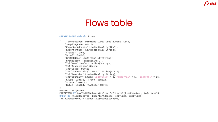
The main table is the flows table. Here is a partial view of it. Many columns are missing. For each Src column, you should have a Dst column. For each InIf column, you have an OutIf column matching. There’s nothing special. We use LowCardinality when it makes sense and the table is ordered by TimeReceived because every queries will use this column.

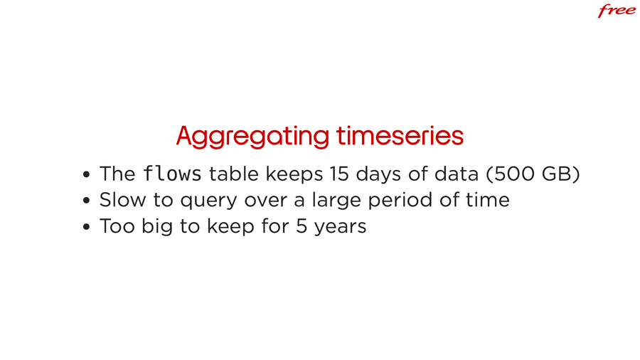
The flows table in our setup keeps 15 days of data. It’s half a terabyte of data. It’s very slow to query for more than one hour of data and almost impossible to query one day, two days, three days. It’s possible but it’s slow. It takes many seconds and we don’t want that. We want an instant response. Also, we want to keep data for five years. This is a common requirement for this kind of setup to be able to look at what happened last year at the same period. To be able to do that we need to aggregate data when it gets older. ClickHouse aggregates data but it was not flexible enough for us.

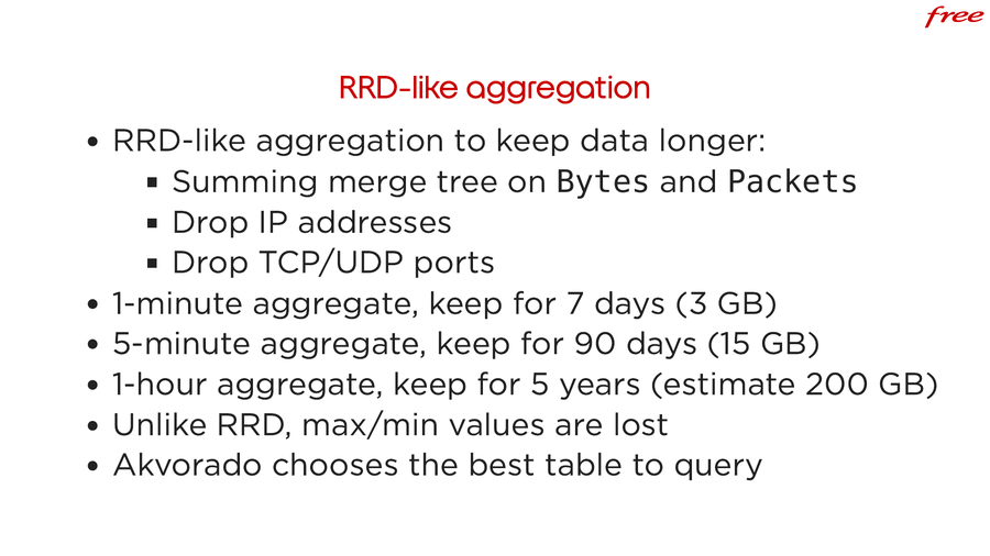
We use an approach inspired by the round-robin database. Round-robin database (RRD) is an ancestor of the time series database. The data is stored in a circular buffer and after some time the data is consolidated using a specific function, mostly max, min, and average. We do that. We use a summing merge tree on bytes and packets. We also drop IP addresses and TCP and UDP ports.

We cannot keep IP addresses for too long for legal reason because it’s personally identifiable information and it’s not that interesting past a few days to know all the IP addresses. The interesting parts of the IP address survive through the network classification. We can attach a region to an IP address for example. Also through the information given by the AS numbers: we know this IP address is owned by Facebook for example. So past a few days, we don’t keep the IP addresses anymore.

TCP and UDP ports, it’s for another reason. We could have kept them but they are very random. Most of the time the source port or the destination port are known, for example port 80 or 443 for HTTP. But the other port is random. So it’s a lot of random data, it’s not easy to know which part is a server port so it’s easier to drop it and again past a few days, it’s not very interesting to keep the ports and it helps compress the data far more, it helps aggregate the data more efficiently to not have that.

Unlike RRD, we don’t keep the maximum values. It’s something that you should do at some point. Because when you zoom out… I can show you on the demo, it would be interesting… When you zoom out, you see it seems that I have the max at 60 Gbps of traffic. But if I ask for the last 30 days instead we see the max is a bit less. It’s because it’s not really a max, it’s an average at the resolution of the table. So an average over five minutes and an average over one hour will give a different maximum value. But that’s something that could be fixable with ClickHouse, I think.

So we have one-minute aggregate table, a five-minute aggregate table, and a one-hour aggregate table. They keep data for seven days, 90 days, and for five years very efficiently. Akvorado automatically chooses the best table depending on the time range, the columns requested (if you request a source IP address or a destination address, you will have to use the main table).

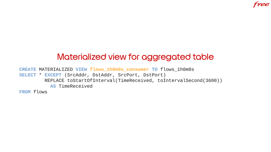
I wanted to show you how we feed data to the aggregated table because it shows a nice feature of ClickHouse. You can select everything with the star except a few columns. So we want to exclude source address, destination address, source port, and destination port. It’s very easy to do that and we can also replace some columns. For example, the TimeReceived is truncated to the previous hour. It’s very nice to be able to do that.

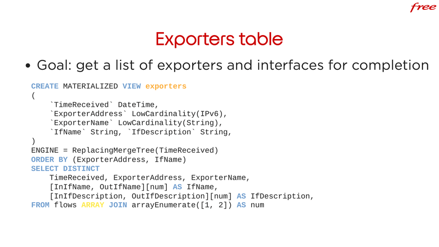
The exporters table. It’s just a small helper table to have a list of exporter names, addresses and interface, names and descriptions and other data. It’s mostly used for completion for completing user input when the user is writing the filter. I wanted to show you that because it’s another nice feature of ClickHouse. You have a lot of ways to manipulate arrays. So with a single query, I can populate the table using ARRAY JOIN and arrayEnumerate.

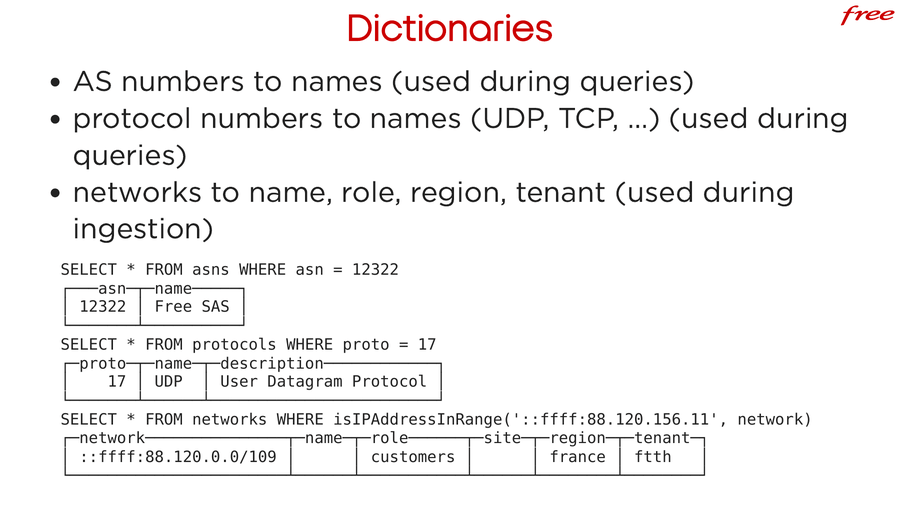
Another interesting part is the dictionaries. We use three dictionaries. One dictionary to map AS numbers to names. There are about 100,000 AS numbers. From one AS number you can get the name.

And we have another dictionary for protocol numbers to names. So protocol number 17 is UDP. The protocol numbers are immutable. AS names change very infrequently. Mostly cosmetic. For example you can have the AS name for Twitch TV can change later to Amazon Twitch TV, but it’s mostly cosmetic and it’s only used for display purpose. So we use these dictionaries during queries.

The third dictionary maps networks, like this, to a name, a role, a region, and a tenant. And this time we use this dictionary during ingestion to materialize some columns because we don’t want historic data to change when you reallocate a subnet to a region.

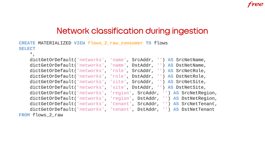
The network classification is done during ingestion using the materialized view where we select everything from what we receive from Kafka and we just add the source net names, source net roles, etc., using the dictionary. The networks dictionary is using the IP_TRIE layout. It means that given an IP Address, ClickHouse is able to do a very fast IP lookup to select the right network.

These are not the only columns generated from other data. If you remember we have also data generated from GeoIP location, from AS numbers and from classification. It’s not done in ClickHouse for GeoIP data. It could have been done in ClickHouse using the same system. It would have worked but it was easy to do that in Akvorado directly. But the classification is done with user-provided rules. So this time it’s easier to do that in the backend. Not in ClickHouse.

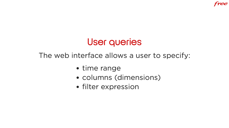
So if you remember the demo, the user inputs a time range, columns, (in the web interface as they are called dimensions) and the filter expression.

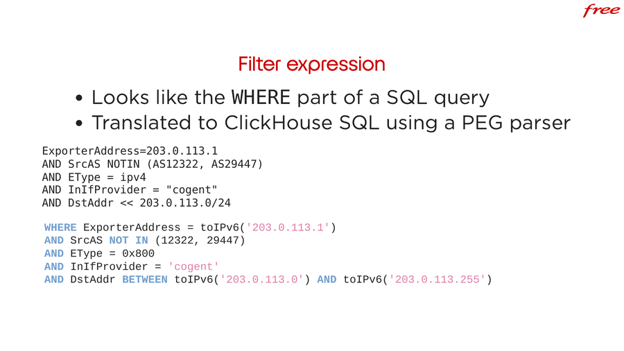
And the filter expression is also something that I find interesting. Our users are network engineers, they may know SQL, but they are not fluent in SQL but they know it well enough that we are using for filters a SQL-like language that we translate to the ClickHouse SQL using a parser.

Our domain is simpler. So we can take shortcuts. We can simplify some aspects. For example the IP address does not need to be quoted. You can use double quotes or single quotes. It doesn’t make a difference. You can use some constant. EType should be an integer but we can give a name in this case. Everything to be easier to use. And the parser will translate that to ClickHouse SQL.

It’s also safe because we parse the filter and then we build the SQL query. If you use an unknown column, you make a syntax error or something like that, the parser will fail with an error message and no query is built. You cannot inject anything in ClickHouse. Even if ClickHouse is not very vulnerable to injection attacks, it’s not possible because the parser needs to understand what you want and it translates that to ClickHouse.

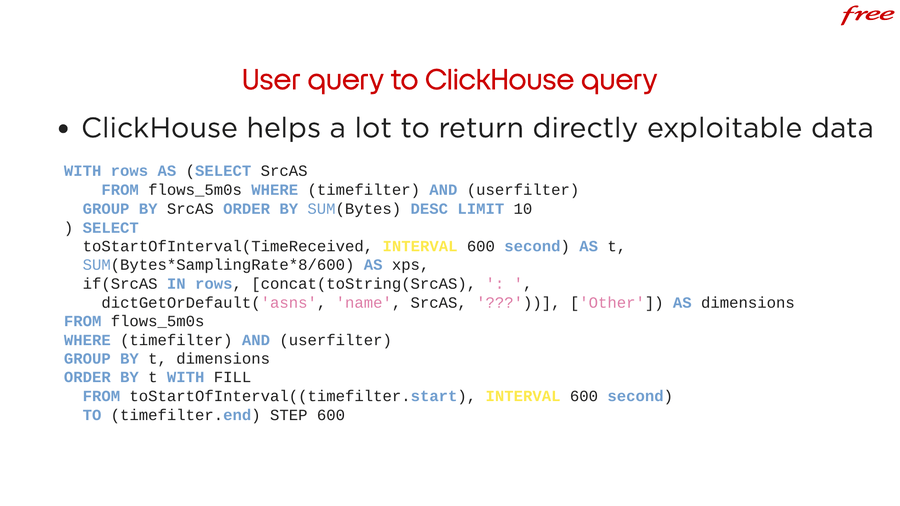
Then the whole user query is translated to ClickHouse SQL. ClickHouse helps a lot to return data that would be directly exploitable by the frontend. For example, when some values are missing, we can fill it automatically with zero values. That’s what is done here.

You notice that I am using the aggregated table with the five-minute aggregation. There is a magic value here which is 600. We adapt the resolution requested by the user, which may be 632 seconds, one value every 632 seconds. We adapt it to match the resolution of the table. It should be a multiple of the resolution of the table for data to look good. So since the resolution is 300 seconds and the user requested about one point every 600 seconds, we will give them one point every 600 seconds.

And there is a subquery. The user requested to get the source AS numbers. We select the top 10 AS numbers matching the query with same time range and the same filter. We will select the top AS numbers. For each AS number that we get, if it’s one of the top 10, we will display the AS number along with its name with the dictionary. Otherwise, we just display Others. This way we don’t have an infinite list of AS numbers returned to the user.

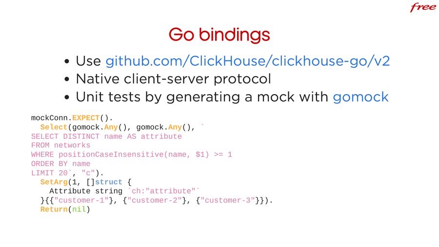
Let’s switch to the back end. It’s written in Go. And we are using clickhouse-go/v2 bindings which is using the native client server protocol. It’s a low level interface but it’s fine for us because abstractions often come with restrictions. The documentation is pretty poor. It’s not up to date with the Go standard but there are a few examples to understand how it works and otherwise it works very well.

We write a lot of unit tests but they are not run against the real database. For each query we provide canned results by using a mock generated with GoMock. For example, during the test, this query is issued. GoMock will generate a fake function that will answer this result: customer-1, customer-2, customer-3. It enables us to do a lot of tests, very fast without relying on an external database.

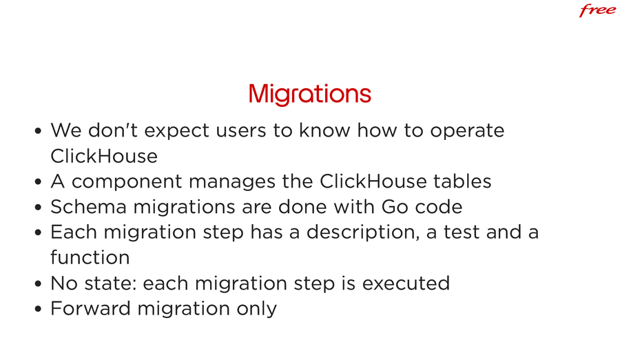
The last thing that I wanted to mention are the migrations. With a regular database, a product often start migrations when you update. For ClickHouse, it may be a bit more complex because you cannot do whatever you want. So we have an orchestrator which manages the different internal and external component, including ClickHouse and Kafka. It manages the schema migrations and it’s done with Go code. Each migration step has a description, a test and a function. There is no state: each migration step is executed on start. And the test says if a step can be skipped or not. It’s only managing forward migrations.

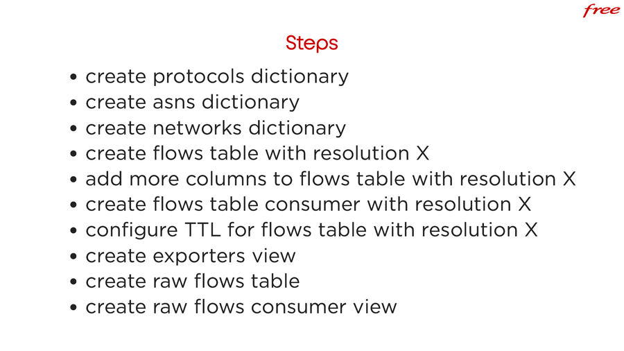
The current steps create dictionaries: protocol, AS numbers, and network dictionary, create the flows tables, the main one and the aggregated ones. If you upgrade from an old schema, there is a step to add the missing columns. There is a step to create consumer flows tables. There is a step to configure the TTL associated with table. This means that if the user configures a different TTL and restarts, the TTLs will be updated. And then a step for the exporters view, the raw flows table, etc.

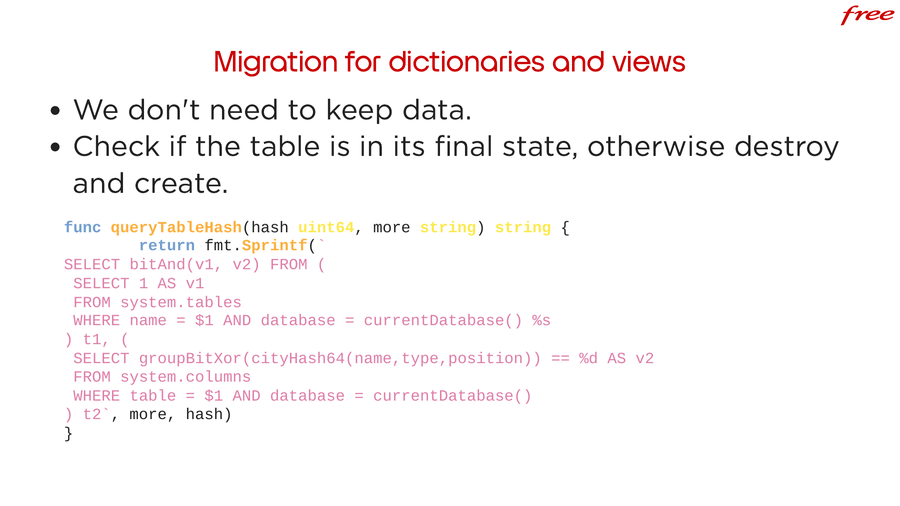
There are two different kinds of steps. The ones that will modify the dictionaries and the views. We don’t need to keep data for this one. We do two checks. We check if the table exists. The table, the view, or the dictionary exists and we check if the table has the right columns at the right positions. So it’s done by hashing the name, type, position from the system columns table and checking against an hard-coded value. So it’s quite nice that ClickHouse exposes a lot of things in the system tables because it enables us to do that.

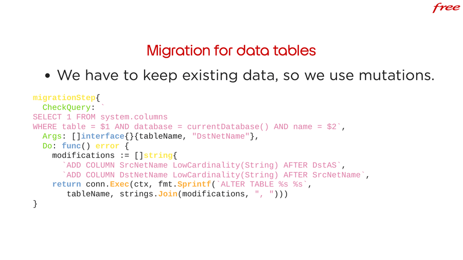
And the second kind of steps that we can have is when we want to keep existing data. So in this case we use mutations. We test “do we have the column that we have to add?” If not then we use ALTER TABLE to add the column. There are many limits of what you can mutate but with some compromises, until today, we were able to do what we wanted to do.

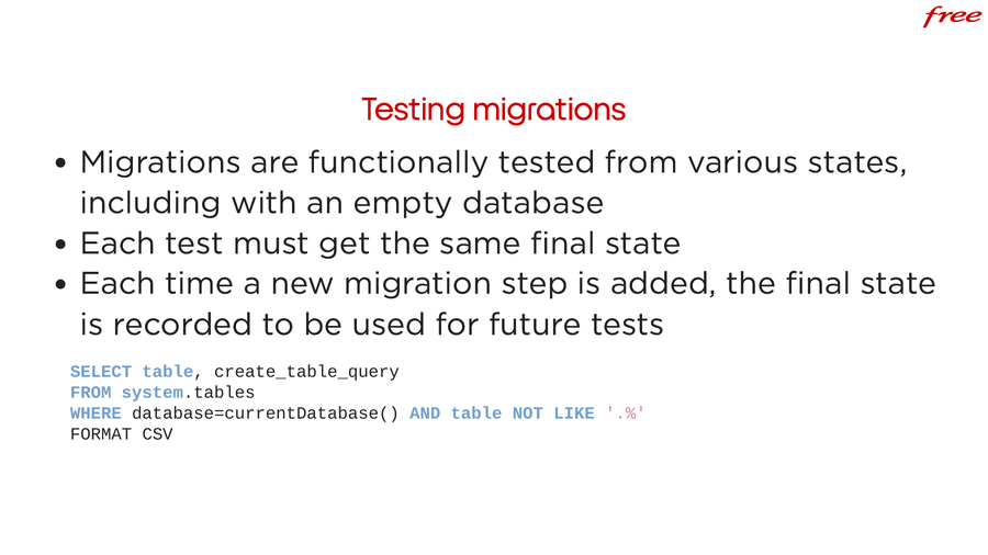
Migrations are tested. They are part of the automatic tests. There is a ClickHouse database spawned in a container and migrations are tested from various states including from an empty database. Each test must get the same final state and each time a migration step is added, the final state is recorded to be used in future tests using the query on the slide. This enables us to ensure that the user is able to migrate from one version to any other version.

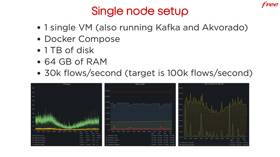
Our setup is quite small. We are running everything on a single VM including Kafka and Akvorado itself. Everything is running in containers using docker-compose. So it’s a very simple setup. One terabyte of disk, 64 GB of RAM. Currently it’s 30,000 flows/s and the target is 100,000 flows/s. You see some usage graph for CPU, memory, and disk. Everything is quite low but there is a DDoS system running in the background, every five seconds, doing requests and it’s the one generating most of the load.

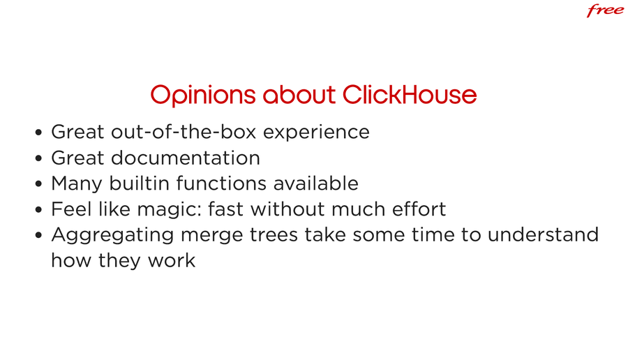
To conclude, my opinions about ClickHouse. It’s a great out of the box experience, great documentation. There are many builtin functions available. String functions that converts to human readable strings. It really feels like that this is something where usability problems are solved directly in ClickHouse instead of having another layer for that. It feels a bit like magic.

Another popular way to do the same thing is to use ElasticSearch. Unlike ElasticSearch, ClickHouse is very fast without much effort and stays very fast. Managing an ElasticSearch cluster is far more difficult for this kind of usage. Aggregating merge tables take some time to understand how they work and it’s easy to do something that looks right but that isn’t. For example if you aggregate using average, you don’t get what you expect. ClickHouse has functions to help you doing that.

So that’s all for me. I welcome a few questions if you want.

Questions#

Vincent, that was an absolutely awesome talk and we do have a couple questions queued up. I can see them. We have a couple from Gilad. So the first one is Akvorado only parses layer three protocols, how does it detect which application it is?

It’s a limitation of using the network protocols NetFlow/IPFIX/sFlow protocols. These flow collector protocols they collect layer 4 information. NetFlow/IPFIX are limited to layer 4 information plus some metadata like the AS numbers. sFlow is able to pick more inside the packets. You can configure it to get the layer 4 headers as well as 200 bytes of each sampled packet. You can do that but currently Akvorado is not using that.

You can guess your application using ports or using IP address. It depends. If for example you have a Kubernetes cluster, the IP address should be able to give you the target application. You can use that. Currently, you don’t know for sure that it’s HTTP, you don’t know which HTTP request was done. Um it’s not this kind of tool, yet.

Cool. The next question from Gilad has my name on it but I can’t really answer it. Gilad said would you suggest having a single table instead of all three tables. Gilad can you just speak up. I think you should be able to talk, you can describe what you had in mind there.

So yes. Now I see you have three tables, one for one-minute aggregation, one for five-minute aggregation, one for one-hour aggregation. Have you tested using one table, with TTL and aggregate one minute old to be five minutes old and five minutes old to be one hour old and all on the same table having one column to identify the bucket size?

Yes. I have tried that but when you aggregate data inside the same table there is a requirement that the primary key… I may be wrong but I didn’t succeed to do that because there is a requirement that the primary key does not change.

In the primary key, we have the TimeReceived and I want to truncate that to the nearest minute, nearest five minutes and nearest hour. I can for example I can have one column with TimeReceived, then I need another column TimeReceived truncated at the minute, TimeReceived truncated at five minutes and TimeReceived truncated at one hour. I need to have the three columns to exist to be able to do the aggregation into the same table and it seems more complex but maybe it would be a better approach. I would be interested to get feedback on that.

Maybe it would have worked, but because it cannot be modified, it means that if I want to add a new kind of aggregation for example, I want to aggregate at 10 minutes, I cannot modify the table to do that because the primary key cannot change. So that’s the main reason that I did go for three tables even if it makes application a bit more complex because you have to select the right table.

So I just want to say that we have a solution close to this and we did one table but we haven’t tested the performance about many tables versus one table. So it was interesting to ask.

Gilad, you had another question which to Vincent, which is how did you deploy ClickHouse, did you use Kubernetes and Vincent, it looked like you were using docker-compose. Did I see that correctly?

Yes, because currently it’s still a bit of a PoC but it’s working so well that we didn’t try to do better. I wasn’t expecting to be able to fit all our data on a single VM. But so currently it’s a bit of proof of concept but it has gone to production this way. So it’s a single VM using docker-compose. You do docker-compose up and you get your working set up and without a lot of memory. So everything is running into containers including ClickHouse. So there is no cluster, it’s a single-node ClickHouse deployment currently.

Cool. Yeah, that’s a great, yeah, that’s a really great example. I have a question. I don’t see any questions on Youtube. If you folks want to ask something, feel free to throw it into the chat. Vincent, I had one. The UI that you have looks really great. How did you build that?

It was a bit of pain because I am not a frontend developer. It is vue.js. This one. It’s this framework. With TailwindCSS. This framework. That’s mostly all. If you want to look, I think it’s explained a bit more in the documentation. It’s open source, you can have a better look. An important component are the graphs. It’s ECharts. It’s an Apache project which is called ECharts. That’s the one handling the graphs and it’s a very great project if you need to do some frontend work with graphs. It’s very robust and very versatile and it took me some time to discover it.

Yeah, it looks awesome and I like the interactivity of it is outstanding. It’s really cool. Good. Is there any other questions to Vincent before we proceed to the next talk? Yes, they have another one. Do you have a plan to parse HTTP? So to investigate Layer 7.

At Free, we are using the NetFlow protocol and the NetFlow protocol doesn’t allow to peak at the layer seven. We would have to use sFlow and we are an internet service provider and we don’t need that. So there is no plan yet. It’s mostly for telco network engineers or datacenter engineers. It could be interesting but no plan.

Nice. Great. Thank you. Alright, thanks for the great questions and I think I don’t see any further questions queued up right now unless I’m missing something. Vincent, thank you so much for a totally awesome talk. This is really enlightening and I think we can stamp you as an honorary database engineer. You did everything great.