In the past week, I ran a lot of benchmarks using a Spirent Avalanche which is an appliance providing performance testing of network related products (a load balancer, a router, a web server, …). The reporting module does not provide a lot of flexibility and the plots are not the most beautiful ones. Fortunately, the results are also exported as CSV.

Matplotlib is a python plotting library which produces great figures without making things hard when they should be easy. It is a good replacement for gnuplot and you don’t need a lot of Python knowledge to use it. The documentation includes a fine user’s guide that should get you started in less than 20 minutes.

Quick introduction#

You can use Matplotlib from IPython to experiment:

$ ipython -pylab
Python 2.6.7 (r267:88850, Jul 10 2011, 08:11:54)
Type "copyright", "credits" or "license" for more information.

  Welcome to pylab, a matplotlib-based Python environment.
  For more information, type 'help(pylab)'.

> In [1]: plot([1,1,4,5,10,11])

When you are ready, you can build a simple Python script:

#!/usr/bin/env python
from matplotlib.pylab import *
plot([1,1,4,5,10,11])
savefig("my-plot.pdf")

Grabbing results from CSV#

Data are contained into a file named realtime.csv. It contains the raw data as well as some general information about the benchmark (test name, description, parameters…). We need to skip them. Fortunately, csv2rec() allows us to load data from a CSV file into a record array and skip the first rows if necessary.

from matplotlib.pylab import *
import sys, os
import gzip

skip = 0
for line in gzip.open(sys.argv[1]):
    if line.startswith("Seconds Elapsed,"):
        break
    skip = skip + 1
ava = csv2rec(gzip.open(sys.argv[1]),skiprows=skip)

Now, the “Elapsed seconds” column can be accessed with ava['elapsed_seconds'].

General structure#

I need 4 plots:

• successful, unsuccessful and attempted transactions per second,
• minimum, average and maximum response time per page,
• Avalanche CPU usage,
• incoming and outgoing bandwidth.

The most important plot is the first one. The second one is less important and the last ones are here only to check we did not hit some bottleneck during the benchmark. We want to produce a page like this:

Matplotlib allows us to plot subfigures. We create 4 subfigures sharing the same X axis (which the number of seconds elapsed since the beginning of the benchmark). We save the result to PDF.

# Create the figure (A4 format)
figure(num=None, figsize=(8.27, 11.69), dpi=100)

ax1 = subplot2grid((4, 2), (0, 0), rowspan=2, colspan=2)
# […]
ax2 = subplot2grid((4, 2), (2, 0), colspan=2, sharex=ax1)
# […]
ax3 = subplot2grid((4, 2), (3, 0), sharex=ax1)
# […]
ax4 = subplot2grid((4, 2), (3, 1), sharex=ax1)
# […]

# Save to PDF
savefig("%s.pdf" % TITLE)

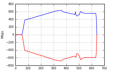
Bandwidth plot#

Let’s start with the easiest plot: bandwidth usage.

# Plot 4: Bandwidth
ax4 = subplot2grid((4, 2), (3, 1), sharex=ax1)
plot(ava['seconds_elapsed'], ava['incoming_traffic_kbps']/1000.,
     'b-', label='Incoming traffic')
plot(ava['seconds_elapsed'], -ava['outgoing_traffic_kbps']/1000.,
     'r-', label='Outgoing traffic')
grid(True, which="both", linestyle="dotted")
ylabel("Mbps", fontsize=7)
xticks(fontsize=7)
yticks(fontsize=7)

Here, in the suplot positioned in (3,1), we plot the number of seconds elapsed versus the incoming traffic with a blue line (b-). We also plot the seconds elapsed versus the outgoing traffic with a red line (r-).

Here is the result:

Most functions of Matplotlib are exposed as a method of the object they refer to and as a global function. In the latest case, the function is applied to the latest created figure or plotting area. For example, plot() is called a function and therefore refer to the plotting area ax4. We could have written ax4.plot() instead.

CPU plot#

The average CPU utilization data available in the CSV file needs to be normalized. We assume the Avalanche to be mostly idle on start. The plotting part is pretty similar to our previous case.

# CPU
max = np.max(ava['average_cpu_utilization'])
order = 10**np.floor(np.log10(max))
max = np.ceil(max/order)*order
cpu = (max - ava['average_cpu_utilization'])*100/max

# Plot 3: CPU
ax3 = subplot2grid((4, 2), (3, 0), sharex=ax1)
plot(ava['seconds_elapsed'],
     cpu,
     'r-', label="Avalanche CPU")
grid(True, which="both", linestyle="dotted")
ylabel("Avalanche CPU%", fontsize=7)
xticks(fontsize=7)
yticks(fontsize=7)

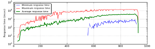
Response time#

We would like to plot response time. We have three corresponding metrics: minimum response time, average response time, maximum response time. Because these metrics start from 0 ms up to several seconds, a logarithmic scale is used:

# Plot 2: response time
ax2 = subplot2grid((4, 2), (2, 0), colspan=2, sharex=ax1)
plot(ava['seconds_elapsed'], ava['minimum_response_time_per_page_msec'],
     'b-', label="Minimum response time")
plot(ava['seconds_elapsed'], ava['maximum_response_time_per_page_msec'],
     'r-', label="Maximum response time")
plot(ava['seconds_elapsed'], ava['average_response_time_per_page_msec'],
     'g-', linewidth=2, label="Average response time")
legend(loc='upper left', fancybox=True, shadow=True, prop=dict(size=8))
grid(True, which="major", linestyle="dotted")
yscale("log")
ylabel("Response time (msec)", fontsize=9)
xticks(fontsize=9)
yticks(fontsize=9)

This is also the first graphic with a legend.

Transactions per second#

The most important plot is the number of transactions per second.

# Plot 1: TPS
ax1 = subplot2grid((4, 2), (0, 0), rowspan=2, colspan=2)
plot(ava['seconds_elapsed'], ava['desired_load_transactionssec'],
     '-', color='0.7', label="Desired Load")
plot(ava['seconds_elapsed'], ava['successful_transactionssecond'],
     'g:', label="Successful")
plot(ava['seconds_elapsed'], smooth(ava['successful_transactionssecond']),
     'g-', linewidth=2)
plot(ava['seconds_elapsed'], ava['attempted_transactionssecond'],
     'b-', label="Attempted")
plot(ava['seconds_elapsed'], ava['aborted_transactionssecond'],
     'k-', label="Aborted")
plot(ava['seconds_elapsed'][:-1], ava['unsuccessful_transactionssecond'][:-1],
     'r-', label="Unsuccessful")
legend(loc='upper left', fancybox=True, shadow=True, prop=dict(size=10))
grid(True, which="both", linestyle="dotted")
ylabel("Transactions/s")

The number of successful transactions is plotted twice: when the benchmarked equipment becomes overloaded, we get a lot of noise in this metric and it can be difficult to read. Therefore, we plot a smoothed version with the help of NumPy:

import numpy as np
def smooth(x, win=4):
    s = np.r_[x[win-1:0:-1],x,x[-1:-win:-1]]
    w = np.ones(win, 'd')
    y = np.convolve(w/w.sum(),s,mode='valid')
    return y[(win-1)/2:-(win-1)/2]

np.r_() is just here to extend our data by the size of the window. np.ones() build a weight vector of the size of the window. If the window is 4, we get [0.25, 0.25, 0.25, 0.25]. We use this vector to apply a convolution to the original data. Here is the result:

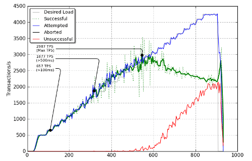
The original data is a green dotted line while the smoothed one is a green thick line. What about the three annotations? Matplotlib allows us to put annotations on a figure. Here is how this is done:

# Noticeable points
count = 0
def highlight(index, reason):
    global count
    if index and index > 0:
        x,y = (ava['seconds_elapsed'][index],
               smooth(ava['successful_transactionssecond'])[index])
        plot([x], [y], 'ko')
        annotate('%d TPS\n(%s)' % (y,reason), xy=(x,y),
                 xytext=(20, -(count+4.7)*22), textcoords='axes points',
                 arrowprops=dict(arrowstyle="-",
                 connectionstyle="angle,angleA=0,angleB=80,rad=10"),
                 horizontalalignment='left',
                 verticalalignment='bottom',
                 fontsize=8)
        count = count + 1

highlight(np.argmax(smooth(ava['successful_transactionssecond'])), "Max TPS")
highlight(np.argmax(cpu > 99), "CPU>99%")
highlight(np.argmax(ava['average_response_time_per_page_msec'] > 500), ">500ms")
highlight(np.argmax(ava['average_response_time_per_page_msec'] > 100), ">100ms")

np.argmax() returns the index of the first maximum value. The trick here is that when I write ava['average_response_time_per_page_msec'] > 100, I get an array with 1 when the value is more than 100 and 0 otherwise. Therefore, np.argmax() will return the first index where the value is superior to 100 ms.

The highlight() function will add a point (plot([x], [y], 'ko')) on the smoothed successful transactions par second plot and add an annotation with some fancy arrow.

Look at this benchmark of nginx as TLS termination for a complete output of this script.